Napathsawan Poopaiboon

Overview

Decision Trees are a non-parametric supervised learning algorithm used for classification and regression. The objective is to learn simple decisions derived from the data features in order to build a model that predicts the value of a target variable. The method builds a flow chart like a tree structure where each internal node represents a feature, each branch denotes an outcome of the test, and each leaf node or terminal node represents a class label. The tree is constructed by recursively creating subsets of the training data depending on the values of the attributes until a stopping requirement is satisfied like the maximum depth of the tree or the minimum number of samples required to a split node.

From the figure above, the tree splits the target variable into different subgroups which are relatively more homogenous from the perspective of the target variable. If the target variable is binary (1 or 0), the decision tree will split the target into subgroups.

Components of a Decision Tree

• A root node: It is the starting point of the decision-making process.
• Decision node: It is a node where the target variable is split again further by other variables.
• Leaf node (Terminal nodes): It is a pure node without any child nodes that indicate a class label or a numerical value.

How Decision Trees Work

The way decision trees work is by separating the data recursively according to various splitting criteria. The objective is to generate consistent subsets of data at every internal node, resulting in accurate predictions at the leaf nodes.

To determine the best features and thresholds for splitting the data, decision trees use different criteria for splitting. These criteria are entropy, gini impurity, and information gain. These metrics aid in the selection of the best features and thresholds that minimize uncertainty or impurity to the greatest extent possible.

The tree starts with the root node. And at each internal node, a decision is applied to determine the appropriate branch to follow. The data is divided into subgroups until it reaches the leaf nodes, which stand for the conclusions or predictions, by using the chosen feature and threshold.

Decision trees partition the data recursively in order to identify relationships and patterns within the dataset. These learned patterns allow the decision tree to make predictions on unseen instances by following the decision path from the root node to the corresponding leaf node.

Attribute Selection Measures

1. Entropy

Entropy is the measure of the degree of randomness in the dataset and how pure a node is. In the case of classification, it calculates the randomness based on the distribution of class labels in the dataset. Entropy is measured by the formula:

Where k is the number of classes for i node.

2. Gini Impurity or Index

Gini impurity is a score that evaluates how accurate a split is among the classified groups. It evaluates a score in the range between 0 and 1 where 0 indicates that all observations belong to a single class and 1 represents a random distribution of the elements within classes. It is a measure of the goodness of the spit in each decision node. It can be measured by the formula:

Where pi is the proportion of elements in the set that belongs to the i category.

3. Information Gain

Information gain measures the reduction in entropy or variance that results from splitting a dataset based on a specific property. It is used in decision tree algorithms to determine the usefulness of a feature by splitting the dataset into more homogeneous groups according to the class labels or target variable. The higher the information gain, the more valuable the feature is in predicting the target variable. It can be calculated by:

Information Gain = Entropy before Splitting – Entropy after Splitting

Information gain quantifies the decrease in variance or entropy that results from splitting the dataset according to attribute A. When creating the decision tree, the splitting criterion is determined by selecting the property that maximizes information gain.

Classification and regression decision trees both leverage information gain. Entropy is used to quantify impurity in classification, whereas variance is used to quantify impurity in regression. All that changes between the two scenarios is that the formula now uses variance or entropy in place of entropy for the information gain computation.

Information Gain Example

The figure below evaluates the information gain of the split class is third class

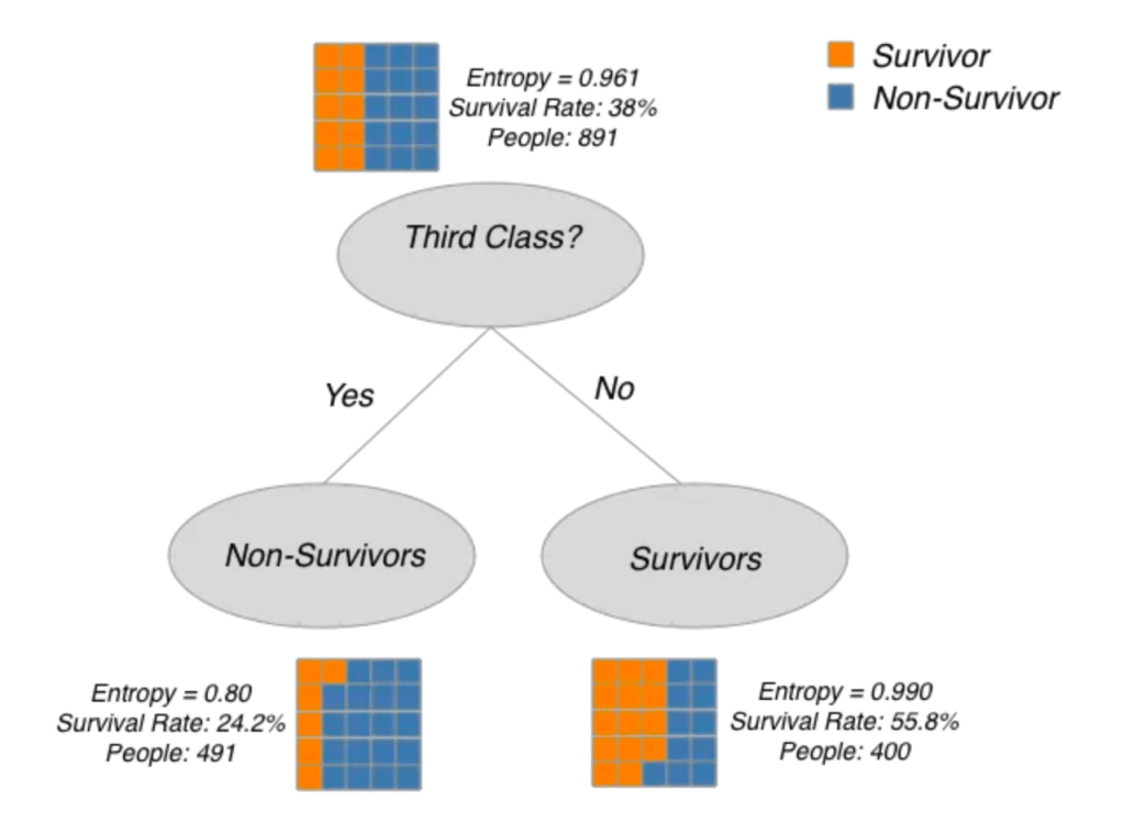
Information Gain = Parent Entropy – Weighted Average (Child Entropy)

= 0.961 – (491*0.8 + 400*0.99)/891

= 0.076

Data Preparation

The data used for clustering analysis is Spotify data. Every row represents a song and every column represents audio features in each song. This data was cleaned already.

The decision tree method is a supervised learning algorithm, this means that it requires labeled data. Some columns were dropped such as artist and track columns. Below is the data before the splitting process. 

The next step after preparing the data is to split the dataset into two subsets: a training set and a testing set. The training set is used to build the decision tree. This is where the model learns patterns, relationships, and features in the data. The model is adjusted and optimized based on this data. It must retain a label, unlike testing set that the label must be removed. However, the testing set is used to evaluate the tree’s performance. In this analysis, the data was split into 70% training set and 30% testing set.

The important thing to note is that although the target variable (y) is removed from the testing set, it is still retained and used for evaluating the model.

Result

There is a key point that is important to know how to interpret the model which is a confusion matrix. The confusion matrix is typically used to assess the performance of a classification model. It is a 2×2 matrix from this analysis that represents the results of a binary classification problem. Each cell in the matrix contains information about the model’s predictions and the actual outcomes. Here is how to interpret the elements of this confusion matrix:

• True Positives (TP): The model correctly predicted positive instances
  (e.g., correctly identified an event as positive). 
• True Negatives (TN): The model correctly predicted negative instances
  (e.g., correctly identified a non-event as negative). 
• False Positives (FP): The model incorrectly predicted positive instances
  (e.g., it predicted an event when there was none). Also known as a Type I error. 
• False Negatives (FN): The model incorrectly predicted negative instances
  (e.g., it failed to identify an event when there was one). Also known as a Type II error.

Moreover, accuracy, precision (positive predictive value), recall (sensitivity, true positive rate), and f-1 score (a balance between precision and recall) can be calculated by the values above.

In this analysis, three different decision trees were built with the goal of explaining the relationship between hit songs and audio features.

The first tree created was fitted without setting any thresholds. And it was created before tuning any hyperparameters. Below are images of the confusion matrix and metrics for classification.

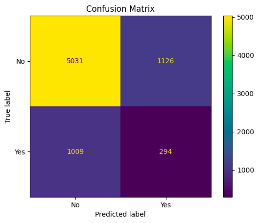
From the confusion matrix:

• 5031 represents the number of true negatives (TN): Instances that are actually in class 0 (negative) and were correctly classified as class 0. 
• 1126 represents the number of false positives (FP): Instances that are actually in class 0 (negative) but were incorrectly classified as class 1 (positive). 
• 1009 represents the number of false negatives (FN): Instances that are actually in class 1 (positive) but were incorrectly classified as class 0 (negative). 
• 294 represents the number of true positives (TP): Instances that are actually in class 1 (positive) and were correctly classified as class 1

And this tree has an accuracy of 71%.

As can be seen from the tree above, it is difficult to dive into it. Therefore, the hyperparameter like the maximum depth in the decision tree was set. To find the best maximum depth, the validation curve and table were created as below.

By carefully looking at the results, we can find the max_depth value where the validation accuracy starts decreasing and the training accuracy starts mounting inordinately. So, max_depth 3 is suitable to be set for the threshold.

The second tree created was trained by using a max depth equal to 3. 

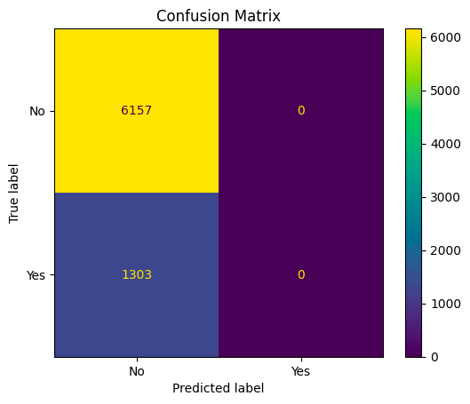
From the results above:

• 6157 represents the number of true negatives (TN): Instances that are actually in class 0 (negative) and were correctly classified as class 0. 
• 0 represents the number of false positives (FP): Instances that are actually in class 0 (negative) but were incorrectly classified as class 1 (positive). 
• 1303 represents the number of false negatives (FN): Instances that are actually in class 1 (positive) but were incorrectly classified as class 0 (negative). 
• 0 represents the number of true positives (TP): Instances that are actually in class 1 (positive) and were correctly classified as class 1

Based on this confusion matrix, the model correctly classified all instances in class 0 (6157 true negatives). However, the model incorrectly classified all instances in class 1, as indicated by the 0 true positives and 1303 false negatives. 

The model has a high specificity (true negative rate) but low sensitivity (true positive rate) for class 1, which suggests that it’s performing well at identifying class 0 instances but not class 1 instances. The class imbalance, where class 0 vastly outnumbers class 1, may be influencing these results. Depending on the specific problem and the relative importance of each class, it may need to be considered strategies for addressing class imbalance or improving the model’s performance for class 1. Althong, the overall accuracy of the model is 83%, the model’s parameters still need tuning.

The last tree created was trained after tuning some parameters which were max depth, min samples split, and min samples leaf. The values adjusted were 10, 7, and 3 respectively. These values were found by using RandomizedSearchCV. It is a function to be used for hyperparameter tuning in machine learning models to find the best parameters in the model. The table below represents the optimization hyperparameters using RandomizedSearchCV.

	Param_dist	Best Parameter
max_depth	[10,20,30,40]	10
min_samples_split	[2,5,7,10]	5
min_samples_leaf	[1,2,3]	2

After the model generated the best parameters, the results are shown as below.

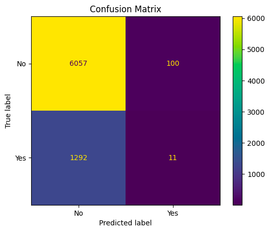
From the results above:

• 6057 represents the number of true negatives (TN): Instances that are actually in class 0 (negative) and were correctly classified as class 0. 
• 100 represents the number of false positives (FP): Instances that are actually in class 0 (negative) but were incorrectly classified as class 1 (positive). 
• 1292 represents the number of false negatives (FN): Instances that are actually in class 1 (positive) but were incorrectly classified as class 0 (negative). 
• 11 represents the number of true positives (TP): Instances that are actually in class 1 (positive) and were correctly classified as class 1

With 81% accuracy, the model is performing well in terms of specificity (correctly identifying actual negatives) and has a decent accuracy. However, it struggles with recall, meaning it has difficulty identifying actual positive instances. This could be indicative of a class imbalance in the dataset or a model that is biased toward the majority class.

Feature Importance

Here is the feature importance scores after tuning parameters. As can be seen from the bar chart above, instrumentalness plays an important role in decision tree model. It has the highest score which is above 0.175, followed by duration and acousticness. However, the score of mood is 0, which means that it has not contributed to the model’s predictions.

Conclusion

This analysis focused on employing decision tree classification with Spotify data to predict hit songs, utilizing a binary label to distinguish between hit and non-hit songs. The models’ performances were evaluated using various metrics such as accuracy, precision, recall, and F1-score. It shows a comprehensive view of how well the model can classify songs as hits or non-hits. Decision trees offer a high level of interpretability. It analyzed the structure of the decision tree to uncover the criteria and musical characteristics that the model relied on when making predictions. This transparency is crucial for artists, producers, and industry stakeholders seeking to understand the factors contributing to song success.

The second tree has the highest accuracy with 83%, however, the model is not performing well, primarily because it is not identifying any instances of the positive class. This could be due to various issues such as class imbalance, model selection, or feature engineering. It is important to address the problem of class imbalance and consider other machine learning algorithms or model adjustments to better predict the positive class. Additionally, evaluating other performance metrics and understanding the problem context is essential for a more comprehensive assessment of model performance.

Moreover, compared to the previous model, this model has a similar accuracy of 81%. The precision has improved in this model, indicating that a higher proportion of predicted positive instances are correct. Also, the recall has also improved compared to the previous model, but it is still quite low. It means that the model is better at identifying some of the actual positive instances but still misses a significant number. This means that this model performs slightly better than the previous one in terms of accuracy, precision, and recall. Further model improvement may be necessary to achieve higher recall while maintaining good precision.

Through the decision tree models created, the importance of various audio features in predicting whether a song will become a hit was determined. This analysis provided a clear understanding of which features significantly influence a song’s success. It can be said that instrumentelness, duration, and acousticness give the best feature importance scores respectively, which means that these three attributes impact the model the most.

To summarize, this analysis represents a significant step in the application of data-driven insights to predict hit songs within the music industry. Through the integration of data analysis, modeling, and interpretation, a tool with practical applications and the potential to influence decision-making processes in the music world have been created. The decision tree has provided valuable business insights, enabling industry stakeholders to better grasp the attributes and patterns associated with hit songs. This understanding can inform marketing strategies, content selection, and resource allocation.