
Overview
A Naive Bayes classifier is supervised learning algorithm that uses probabilistic methods for classification task. The algorithm is based on the Bayes theorem with an independence assumption among predictors. This method is based on the assumption that the attributes of the input data are independent of each other given the class which enables the algorithm to produce precise and fast predictions.

Using the Bayes Theorem, the probability of A happening can be found, given that B has occurred. Here, B is the evidence and A is the hypothesis. In this formular, the independence of the predictors and features is assumed. That is presence of one particular feature does not affect the other, so it is called naive.
Laplace Smoothing in Naive Bayes Algorithm
Laplace smoothing is a smoothing technique that handles the problem of zero probability in Naive Bayes. If a given token and class never occur together in the training data, then the probability estimate for that token conditioned on that class will be zero. It is particularly useful when dealing with categorical data and text classification tasks.
In the context of Naive Bayes, laplace smoothing is applied to handle the situation where a feature or attribute has a count of zero for a particular class. This can lead to zero probabilities, which can cause issues when calculating probabilities using Bayes’ theorem. Laplace smoothing helps to prevent zero probabilities by adding a small constant to each count.
Example
Here is an example of text classification where the task is to classify whether the review is positive or negative. A likelihood table based on the training data is built and the table values were used for querying a review.
Query review = w1 w2 w3 w’
Where w’ is a word in a review is not present in the training dataset
There are four words in the query review, and only w1, w2, w3 are present in the training set. So, we have a likelihood of those three words. To calculate whether the review is positive or negative, we will compare P(positive | review) and P(negative | review).

In the likelihood table, we know likelihood values of P(w1|positive), P(w2|Positive), P(w3|Positive), and P(positive) but there is no likelihood of P(w’ | positive).
If the word is absent in the training set:
- Assigning it a value of 1, which means the probability of w’ occurring in positive P(w’|positive) and negative review P(w’|negative) is 1
- Laplace Smoothing

Where α is the smoothing parameter
K is the number of dimensions (features) in the data
N is the number of reviews with y = positive
If α is not equal to 0, it means that the probability will no longer be zero even if a word is not present in the training dataset.
Multinomial Naive Bayes
The Multinomial Naive Bayes classifier is suitable for classification with discrete features. It is an algorithm that is useful for text classification problems in natural language processing. It is especially helpful, when dealing with text data that has distinct properties, such word frequency counts. The distribution is parametrized by vectors θy = (θy1, … , θyn) for each class y, where n represents the number of features and θyi represents the probability P(xi | y) of feature i appearing in a simple belonging to class y.
Bernoulli Naive Bayes
The Bernoulli Naive Bayes is a part of the family of naive bayes. It only takes binary values. The most common example is when determine whether or not a word that exists in a document will be included in each value. The algorithm is for the data that is distributed according to multivariate bernoulli distribution. Although there may be multiple features, each one is assumed to be a binary value variable.
The decision rule for bernoulli naive bayes is based on

This is not the same as the multinomial NB’s rule in that it penalizes explicitly the absence of a feature i that serves as an indication for class y, whereas the multinomial variation would just ignore the absence of a feature.
Data Preparation
The data used for clustering analysis is Spotify data. Every row represents a song and every column represents audio features in each song. This data was cleaned already.

The naive bayes method is a supervised learning algorithm, this means that it requires labeled data. Some columns were dropped such as artist and track columns. Below is the data before the splitting process. The data used was the normalized data.

The next step after preparing the data is to split the dataset into two subsets: a training set and a testing set. The training set is used to build the decision tree. This is where the model learns patterns, relationships, and features in the data. The model is adjusted and optimized based on this data. It must retain a label, unlike testing set that the label must be removed. However, the testing set is used to evaluate the tree’s performance. In this analysis, the data was split into 70% training set and 30% testing set.


The important thing to note is that although the target variable (y) is removed from the testing set, it is still retained and used for evaluating the model.
Result
The confusion matrix is typically used to assess the performance of a classification model. It is a 2×2 matrix from this analysis that represents the results of a binary classification problem. Each cell in the matrix contains information about the model’s predictions and the actual outcomes. Here is how to interpret the elements of this confusion matrix:
- True Positives (TP): The model correctly predicted positive instances
(e.g., correctly identified an event as positive). - True Negatives (TN): The model correctly predicted negative instances
(e.g., correctly identified a non-event as negative). - False Positives (FP): The model incorrectly predicted positive instances
(e.g., it predicted an event when there was none). Also known as a Type I error. - False Negatives (FN): The model incorrectly predicted negative instances
(e.g., it failed to identify an event when there was one). Also known as a Type II error.
Moreover, accuracy, precision (positive predictive value), recall (sensitivity, true positive rate), and f-1 score (a balance between precision and recall) can be calculated by the values above.
- Accuracy: The number of correct predictions over all predictions
- Precision: A measure of how many of the positive predictions made are correct (true positives).
- Recall (Sensitivity): A measure of how many of the positive cases the classifier correctly predicted, over all the positive cases in the data.
- F1-score: The harmonic mean of precision and recall. It provides a balanced measure that considers both false positives and false negatives.
- Support: The number of actual occurrences of each class in the dataset. It represents the number of instances in each class.
The Naive Bayes Classifier was effective for classifying hit and non-hit songs. The multinomial naive bayes was applied, and the results are shown as below.
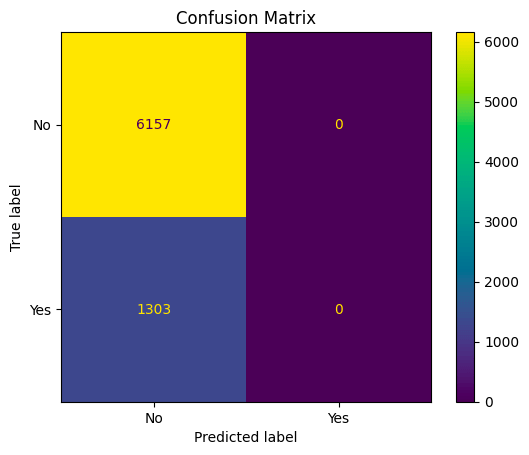

From the results above:
- 6157 represents the number of true negatives (TN): Instances that are actually in class 0 (negative) and were correctly classified as class 0.
- 0 represents the number of false positives (FP): Instances that are actually in class 0 (negative) but were incorrectly classified as class 1 (positive).
- 1303 represents the number of false negatives (FN): Instances that are actually in class 1 (positive) but were incorrectly classified as class 0 (negative).
- 0 represents the number of true positives (TP): Instances that are actually in class 1 (positive) and were correctly classified as class 1
Accuracy measures the overall correctness of the model’s predictions. The overall accuracy is 0.83, which means the model is correct in its predictions for 83% of the instances. However, this metric can be misleading in imbalanced datasets, as high accuracy can result from correctly classifying the majority class while completely missing the minority class.
Note
TP (True Positives) is 0: This means that the model correctly identified 0 songs as hit (positive) out of the actual 1303 hit songs. In other words, the model did not successfully classify any of the actual hit songs correctly.
FP (False Positives) is 0: This means that the model did not incorrectly classify any non-hit songs as hit. In other words, there were no false alarms where the model mistakenly classified a non-hit song as a hit.
The reason both TP and FP are zero suggests that the model’s classification for the hit songs class (positive class) was not effective. It did not identify any of the actual hit songs correctly, and it also did not mistakenly classify any non-hit songs as hit.
Conclusion
The Multinomial Naive Bayes model was used to categorize songs as hit or non-hit based on the available dataset and its attributes. Several criteria were used to assess the model’s performance, including accuracy, precision, recall, and F1-score.
The model achieved an accuracy of roughly 83%, implying that it is capable of correctly identifying a major number of the songs as hit or non-hit. It is important to highlight, however, that the model’s performance is not totally good, as evidenced by other metrics.
Moreover, the precision for the hit class is low, implying that the model may produce a high number of false positives. This means that some songs that are not hit may be mistakenly labeled as such. The recall for the hit class, on the other hand, is likewise poor, indicating that the model may miss many true hit (high false negatives). The F1-score, which balances precision and recall, is rather low, indicating that the model’s overall performance might be improved.
In conclusion, while the Multinomial Naive Bayes model shows potential for classifying songs as hit or non-hit, it may not be the most suitable model for this particular task. The results suggest that there is room for optimization and further exploration of different machine learning algorithms and feature engineering techniques. The low precision and recall for the hit class are areas of concern that should be addressed to enhance the model’s performance.
