
Overview
Support Vector Machine (SVM) is a supervised machine learning algorithm that works best on smaller datasets but on complex ones. It can be useful for both regression and classification tasks but works best in classification problems. The objective of this algorithm is to find a hyperplane in an N-dimensional space (N refers to the number of features) that distinctly classifies the data points.

Maximizing the margin distance is considered optimal. This is because it provides some reinforcement so that the data points can be classified with more confidence.
Types of Suport Vector Machine Algorithms
- Linear SVM
Only when the data is perfectly linearly separable, we can use Linear SVM. The data points are perfectly linearly separable if they can be divided into two classes using a single straight line (if 2D).
- Non-Linear SVM
Non-Linear Support Vector Machines (SVM) can be applied when the data is not linearly separable. In other words, if the data points cannot be classified into two classes using a straight line (assuming the data is two-dimensional), sophisticated techniques such as kernel tricks can be applied. Since linearly separable data points are uncommon in real-world applications, kernel tricks are used to solve them.

- Support Vectors: The points that are nearest to the hyperplane. A separating line will be defined with the help of these data points.
- Margin: It is the distance between the observations called support vectors that are closest to the hyperplane. A large margin is a good margin.
How does Support Vector Machine work?
Suppose there are two independent variables, x1 and x2, and one dependent variable as either a blue or a red circle.

To classify these points, we need to choose the best line or the best hyperplane that segregates the data points, and the hyperplane that distance from it to the nearest data point on each side is maximized will be chosen. This can be done by finding different hyperplanes that classify the labels in the best way, then it will choose the one that is furthest from the data points or the one that has a maximum margin. A hyperplane that satisfies this condition is referred to as the maximum-margin hyperplane or hard margin. From the figure above, the hyperplane chosen is L2.
What if there is one blue ball in the boundary of the red balls as it is shown below?
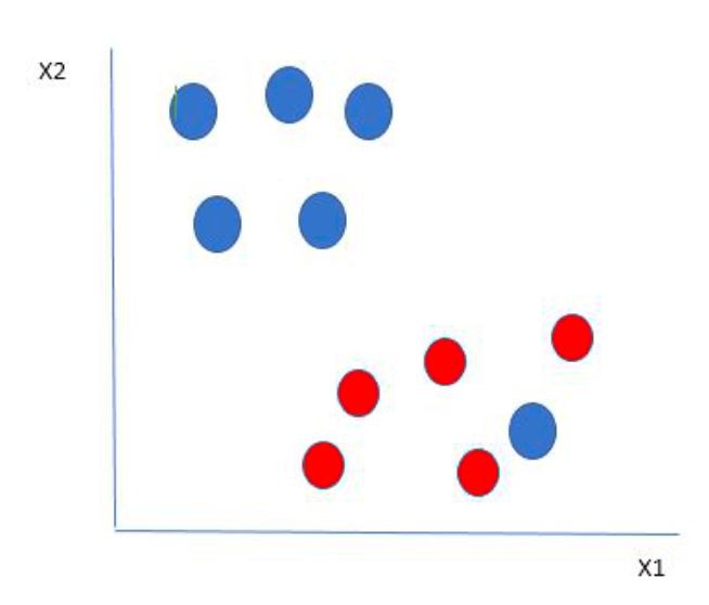
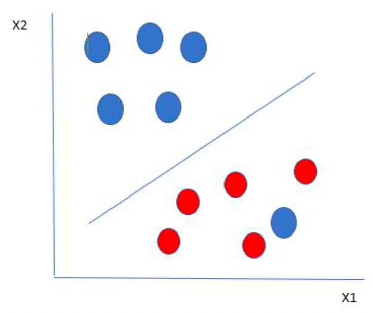
The blue ball in the boundary of red balls is an outlier of blue balls. However, the SVM algorithm’s features allow it to identify the optimal hyperplane that maximizes the margin while ignoring the outlier. SVM determines the maximum margin for this kind of data point, just like it did for earlier data sets, and it also adds a penalty each time a point crosses the margin. These kinds of margins are hence referred to as soft margins. If there is a soft margin to the dataset, the SVM will try to minimize it. But when the data do not separate linearly, what should be done?

From the figure above, the SVM algorithm uses a kernel to create a new variable in order to address this problem. As a function of the distance from the origin (o), we designate a new variable yi and call a point xi on the line. If we plot this, the result is as follows.

In this instance, the distance from the origin determines the creation of the new variable, y. A kernel is a non-linear function that generates a new variable.
Kernel Functions in Support Vector Machine
A kernel function is a technique for taking input data and transforming it into the format needed for data processing. The term “kern” refers to a group of mathematical operations that Support Vector Machine uses to provide a window for data manipulation. Thus, the training set of data is typically transformed using a kernel function to enable a non-linear decision surface to turn into a linear equation in a greater number of dimension spaces. In essence, it gives back the ordinary feature dimension’s inner product of two points. There are two popular kernels that always are applied in the model polynomial kernel and gaussian radial basis function or RBF kernel.
- Polynomial Kernel SVM
Polynomial Kernel SVM uses a polynomial function to transform the input data into a higher dimensional space. The polynomial kernel function raises the result to a power determined by the function’s degree parameter after adding a constant to the dot product of the input data points. The result of this transformation is a set of new features that represent the non-linear relationships between the input data.
- Gaussian RBF kernel
RBF is more complex and efficient than polynomial kernel functions. It can combine multiple polynomial kernels multiple times of different degrees to project the non-linearly separable data into higher dimensional space so that it can be separable using a hyperplane. The RBF kernel performs the classification using the fundamental concepts of Linear SVM after mapping the data into a high-dimensional space by calculating the dot products and squares of each feature in the dataset.
Data Preparation
The data used for the support vector machine is Spotify data. Every row represents a song and every column represents audio features in each song. This data was cleaned already.

The support vector machine method is a supervised learning algorithm, this means that it requires labeled data. Some columns were dropped such as artist and track columns. Since there are many rows in the dataset, we chose to use 5000 rows in the model. Below is the data before the splitting process. The data used was the normalized data.

The next step after preparing the data is to split the dataset into two subsets: a training set and a testing set. The training set is used to build the decision tree. This is where the model learns patterns, relationships, and features in the data. The model is adjusted and optimized based on this data. It must retain a label, unlike testing set that the label must be removed. However, the testing set is used to evaluate the tree’s performance. In this analysis, the data was split into 70% training set and 30% testing set.


The important thing to note is that although the target variable (y) is removed from the testing set, it is still retained and used for evaluating the model.
Results
The confusion matrix is typically used to assess the performance of a classification model. It is a 2×2 matrix from this analysis that represents the results of a binary classification problem. Each cell in the matrix contains information about the model’s predictions and the actual outcomes. Here is how to interpret the elements of this confusion matrix:
- True Positives (TP): The model correctly predicted positive instances (e.g., correctly identified an event as positive).
- True Negatives (TN): The model correctly predicted negative instances (e.g., correctly identified a non-event as negative).
- False Positives (FP): The model incorrectly predicted positive instances (e.g., it predicted an event when there was none). Also known as a Type I error.
- False Negatives (FN): The model incorrectly predicted negative instances (e.g., it failed to identify an event when there was one). Also known as a Type II error.
Moreover, accuracy, precision (positive predictive value), recall (sensitivity, true positive rate), and f-1 score (a balance between precision and recall) can be calculated by the values above.
- Accuracy: The number of correct predictions over all predictions
- Precision: A measure of how many of the positive predictions made are correct (true positives).
- Recall (Sensitivity): A measure of how many of the positive cases the classifier correctly predicted, over all the positive cases in the data.
- F1-score: The harmonic mean of precision and recall. It provides a balanced measure that considers both false positives and false negatives.
- Support: The number of actual occurrences of each class in the dataset. It represents the number of instances in each class.
The SVM models were trained with three different kernels: Linear, RBF, and Polynomial. GridSearchCV was applied to find the best parameter in each kernel. C = 0.1, 1, 10, and 100 were candidates to find the best model.
Linear Kernel
The GridSearchCV function had the best performance with candidate C = 0.1 which gave a score of 0.7059 when using the linear kernel.
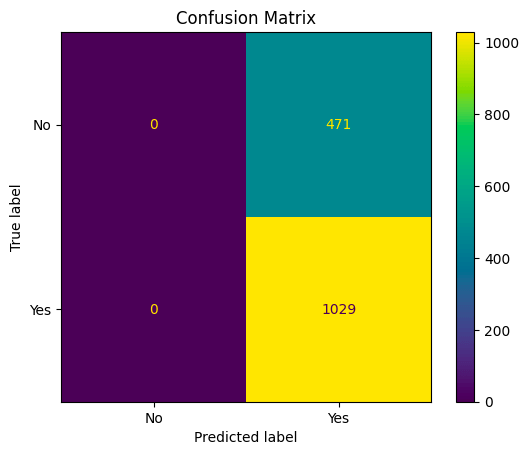

From the confusion matrix:
- 0 represents the number of true negatives (TN): Instances that are actually in class 0 (negative) and were correctly classified as class 0.
- 471 represents the number of false positives (FP): Instances that are actually in class 0 (negative) but were incorrectly classified as class 1 (positive).
- 0 represents the number of false negatives (FN): Instances that are actually in class 1 (positive) but were incorrectly classified as class 0 (negative).
- 1029 represents the number of true positives (TP): Instances that are actually in class 1 (positive) and were correctly classified as class 1
This confusion matrix suggests that the model is predicting only the positive class (hit) and is not making any negative class predictions (non-hit). The accuracy might be misleadingly high because it does not consider the actual distribution of classes. The recall is equal to 1 which is high because it correctly identifies all positive instances but at the cost of not identifying any negative instances. The precision is also equal to accuracy, and the F1 score indicates a balance between precision and recall.
In practical terms, this means that if a balance between hit and non-hit predictions is needed, the model may need to be adjusted because it is too biased towards predicting the positive class.
RBF Kernel
The GridSearchCV function had the best performance with candidate C = 10 which gave a score of 0.7097 when using the RBF kernel.
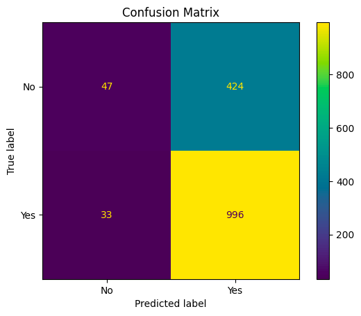

From the confusion matrix:
- 47 represents the number of true negatives (TN): Instances that are actually in class 0 (negative) and were correctly classified as class 0.
- 424 represents the number of false positives (FP): Instances that are actually in class 0 (negative) but were incorrectly classified as class 1 (positive).
- 33 represents the number of false negatives (FN): Instances that are actually in class 1 (positive) but were incorrectly classified as class 0 (negative).
- 996 represents the number of true positives (TP): Instances that are actually in class 1 (positive) and were correctly classified as class 1
From the confusion matrix, the RBF kernel indicates a more balanced performance compared to the linear one. The accuracy is decent and both precision and recall are reasonable. Also, the F1 score provides a balanced measure considering both precision and recall.
Polynomial Kernel
The GridSearchCV function had the best performance with candidate C = 100 which gave a score of 0.7114 when using the polynomial kernel.


The result shows a similar pattern as the RBF one, with decent accuracy, recall, and F1 score. However, the GridSerchCV score for the polynomial kernel is higher than the linear and RBF kernels.
Conclusion
In this analysis, we applied a Support Vector Machine (SVM) to analyze the Spotify dataset with the target variable being the classification of songs into hit or non-hit songs. The goal of this analysis was to build a robust prediction model distinguishing between hit and non-hit songs based on various features extracted from the dataset.
After building models with three different kernels which are Linear, RBF, and Polynomial kernels, the final model achieved a commendable accuracy score of 0.70 which is a model using a polynomial kernel. The matrix serving as a comprehensive evaluation tool reflects the model’s ability to correctly classify instances of true positives and true negatives.
In conclusion, the use of Support Vector Machines on the Spotify dataset has proven effective in predicting the hit or non-hit status of songs. The refined model achieved promising accuracy, demonstrating its potential for real-world applications in music analytics. This study contributes to the growing body of knowledge in the intersection of machine learning and music analysis, highlighting SVM as a valuable tool for predicting song success in the context of Spotify data.
